Tennis court line detector: Part 2, training a CNN

Synthetic data settings

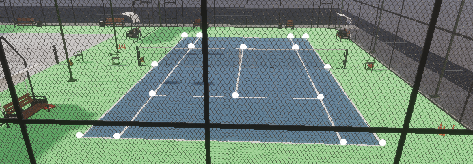
To recap part 1, we built a synthetic data generator for tennis courts with labeled keypoints.  

with corresponding annotations in the SOLO JSON format.  

Here are the randomizer settings:

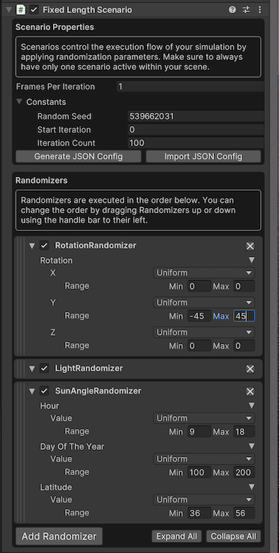
Note that the rotation randomizer only makes relatively small rotations to spin the court on the y axis by -45 to 45 degrees.  This is to keep the problem easy for the first iteration.  This constrained rotation keeps the "front" keypoints in the front of the images, and the "back" keypoints in the back of the image, otherwise the network may have problems converging.  If it was rotated 180 degrees, the data generator would somehow have to flip the keypoints, which seems difficult.

There are a few lighting randomizers, and note that only 100 images are generated.

Deciding on an architecture

Let's start with a simple architecture: VGG16 pre-trained on ImageNet.

We'll remove the VGG16 final layer with 1000 outputs and replace it with a fully connected layer (head) that has 16 * 2 outputs.  For each keypoint:

1. X position
2. Y position

Later we'll generate harder images where some keypoints aren't visible, and add a "Visibility Status" output for training and prediction.

Defining the model

To begin with, we'll try to overfit the model on the training data, as described in Andrej Karpathy's A Recipe for Training Neural Networks.  Since we're trying to overfit, for now we'll remove all regularization, such as dropout layers.  Later when trying to regularize, we'll look into re-adding these.

To avoid having to deal with bugs in training loop code, define the model in a pytorch lightning module.

class LitVGG16(pl.LightningModule):
    
    def __init__(self, num_epochs):

        super().__init__()

        self.num_epochs = num_epochs
        
        # Create a VGG16 network
        self.vgg16 = torch.hub.load('pytorch/vision:v0.6.0', 'vgg16', pretrained=True)

        # x,y coordinates of the 16 keypoints
        num_out_features = 16 * 2

        # Freeze the weights of all the CNN layers
        for param in self.vgg16.features.parameters():
            param.requires_grad = False

        # Redefine the classifier to remove the dropout layers
        self.vgg16.classifier = nn.Sequential(
            nn.Linear(25088, 4096),
            nn.ReLU(inplace=True),
            nn.Linear(4096, 4096),
            nn.ReLU(inplace=True),
            nn.Linear(4096, num_out_features)
        )

    def forward(self, x):
        y_pred = self.vgg16(x)
        return y_pred
    
    def training_step(self, batch, batch_idx):
        x, y = batch
        y_pred = self(x)
        loss = torch.nn.functional.mse_loss(y_pred, y)
        self.log('train_loss', loss, prog_bar=True)

        # Log the learning rate
        scheduler = self.lr_schedulers()
        current_lr = scheduler.get_last_lr()[0]        
        self.log("learning_rate", current_lr, prog_bar=True)

        return loss
    
    def configure_optimizers(self):
        
        optimizer = optim.Adam(self.parameters(), lr=1e-3)

        # Define a learning rate scheduler
        scheduler = optim.lr_scheduler.CosineAnnealingLR(
            optimizer, 
            T_max=self.num_epochs, 
            eta_min=1e-5 
        )

        return [optimizer], [scheduler]

Building a pytorch dataset

Since the annotations are generated in the SOLO JSON  format, we'll need a custom dataset that knows how to read this format.

class TennisCourtDataset(torch.utils.data.Dataset):

    def __init__(self, data_path, transform=None):
        
        self.data_path = data_path

        solo = Solo(data_path=data_path)

        # Preload all frames to allow for random access
        self.solo_frames = [frame for frame in solo.frames()]

    def __len__(self):
        return len(self.solo_frames)

    def __getitem__(self, idx):
        
        solo_frame = self.solo_frames[idx]

        # Each frame has a list of a single capture
        capture = solo_frame.captures[0]

        # Figure out the filepaths for the image
        sequence = solo_frame.sequence
        capture_img_file_path = f"sequence.{sequence}/{capture.filename}"

        # Load the image and convert it to the appropriate tensor
        img_tensor, img_size = TennisCourtImageHelper.imagepath2tensor(
            self.data_path, 
            capture_img_file_path, 
            TennisCourtImageHelper.img_rescale_size
        )

        # Get a reference to the keypoint annotations
        annotations = capture.annotations
        keypoint_annotations = annotations[0]
        keypoints = keypoint_annotations.values[0].keypoints
        if len(keypoints) != 16:
            raise Exception("Expected 16 keypoints")
        
        # Extract the x,y values into a nested list
        keypoint_tuples = [
            (kp.location[0], kp.location[1]) for kp in keypoints
        ]

        # Rescale the keypoints to match the rescaled image
        rescaled_keypoints = TennisCourtImageHelper.rescale_keypoint_coordinates(
            keypoint_tuples, 
            img_size, 
            TennisCourtImageHelper.img_rescale_size
        )

        # Flatten the nested list
        flattened_rescaled_keypoints = [
            element for sublist in rescaled_keypoints for element in sublist
        ]

        # Convert the list to a tensor
        keypoints_tensor = torch.tensor(flattened_rescaled_keypoints)
        
        return img_tensor, keypoints_tensor

The full code including the helper functions are available in https://github.com/tleyden/tennis_court_cnn

A few notes on the above snippet:

1. The image is resized to 224 x 224
2. The keypoints are extracted and then rescaled to match the target image size of 224 x 224.  Without this, the keypoints will be in the wrong place in the image!

Train the model

dataset = TennisCourtDataset(data_path=data_path)

# Create the dataloader and specify the batch size
train_loader = utils.data.DataLoader(
    dataset, 
    batch_size=32, 
    shuffle=True
)

# Create the lightning module
litvgg16 = LitVGG16(num_epochs=50)

trainer = pl.Trainer(
    callbacks=[checkpoint_callback],
    max_epochs=num_epochs, 
    logger=wandb_logger, 
    log_every_n_steps=10    
)
trainer.fit(model=litvgg16, train_dataloaders=train_loader)

Add visualization to wandb logging

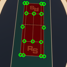
In order to visualize how the network is performing, let's draw both the ground truth and predicted keypoints on top of the image using opencv.

    @staticmethod
    def add_keypoints_to_image(pil_image: Image, kps: List[float], color: tuple[int]) -> Image:

        # Convert each float -> int
        kps = [int(round(kp)) for kp in kps]
        
        # Convert the flattened keypoints to a list of tuples
        keypoint_pairs = [
            (kps[i], kps[i + 1]) for i in range(0, len(kps), 2)
        ]

        # Convert the image to opencv format
        opencv_image = cv2.cvtColor(
            np.array(pil_image), cv2.COLOR_RGB2BGR
        )

        for keypoint_pair in keypoint_pairs:
            center_coordinates = keypoint_pair  # (x, y) coordinates of the center
            thickness = 2  # Thickness of the circle's outline
            radius = 5  # Radius of the circle
        
            # Draw the circle on the image
            cv2.circle(opencv_image, center_coordinates, radius, color, thickness)

        # Convert the image back to PIL format
        pil_image = Image.fromarray(
            cv2.cvtColor(opencv_image, cv2.COLOR_BGR2RGB)
        )

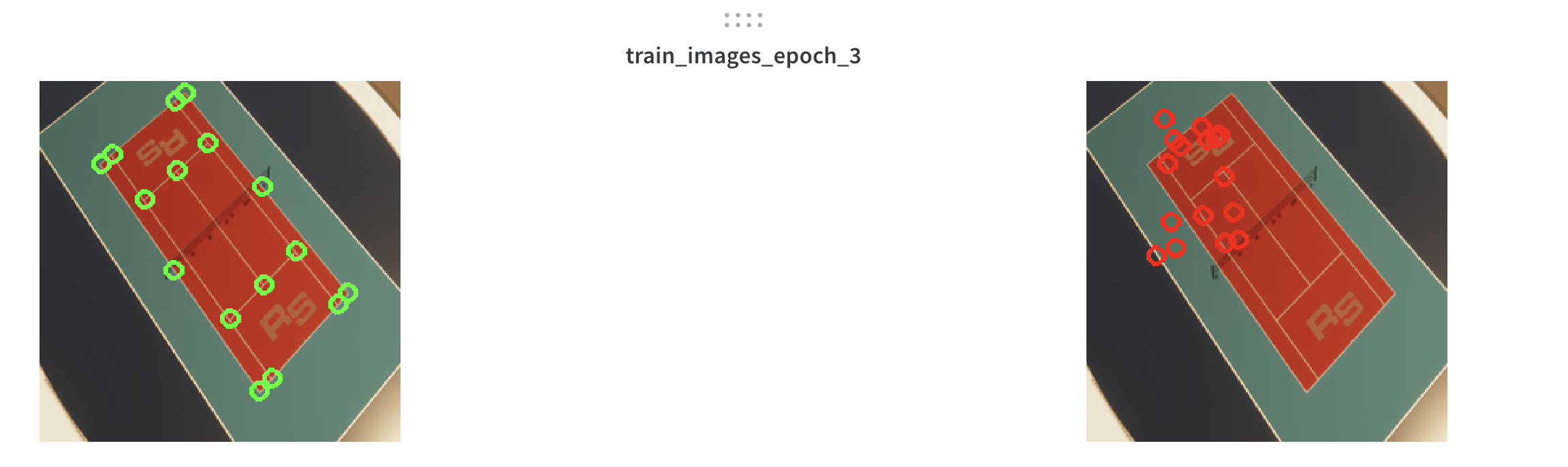
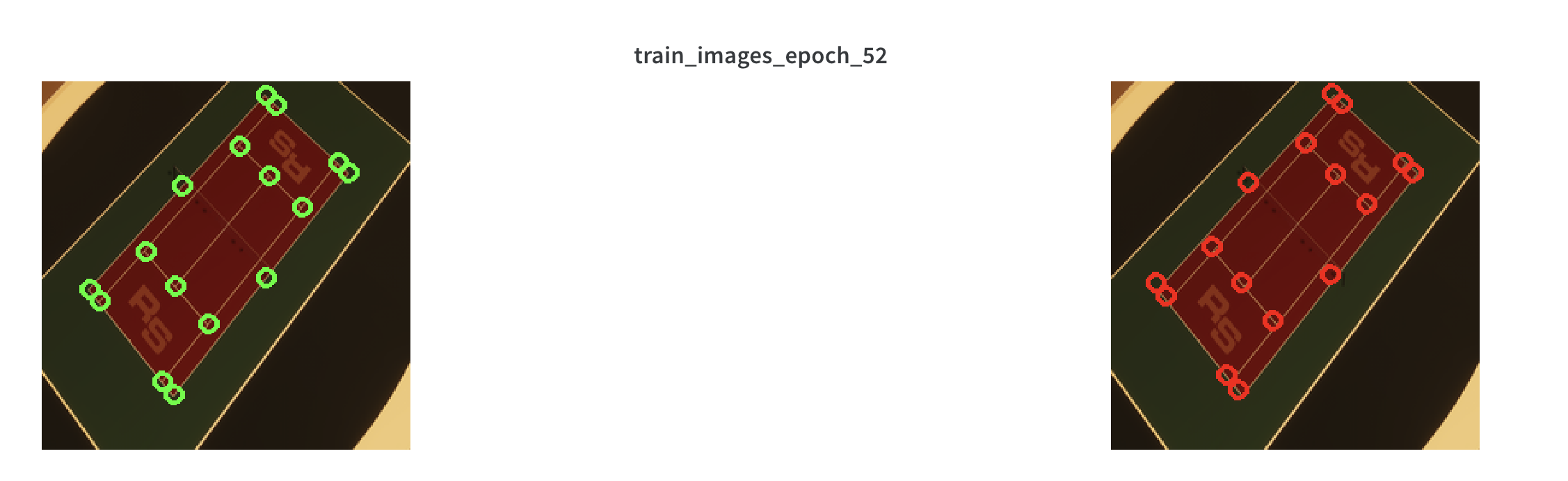
        return pil_image

and during training, log two separate images with the ground truth and predicted keypoints projected to wandb media:

def training_step(self, batch, batch_idx):
    
    .. snip ..

    # Log the first image of the first batch of each epoch
    if batch_idx == 0:

        first_img_in_batch = x[0]

        # Convert the tensor to a PIL image
        pil_image = ToPILImage()(first_img_in_batch)
        
        # Show green keypoints for the ground truth and red keypoints for the predicted keypoints
        pil_image_ground_truth = add_keypoints_to_image(
            pil_image, y[0].tolist(), color=(0, 255, 0)
        )
        pil_image_predicted = add_keypoints_to_image(
            pil_image, y_pred[0].tolist(), color=(0, 0, 255)
        )
        
        wandb.log(
            {f"train_images_epoch_{self.current_epoch}": 
             [wandb.Image(pil_image_ground_truth), wandb.Image(pil_image_predicted)]}
        )

    return loss

Now when training, the wandb UI will visually show the network learning:

Run the training + analyzing the result

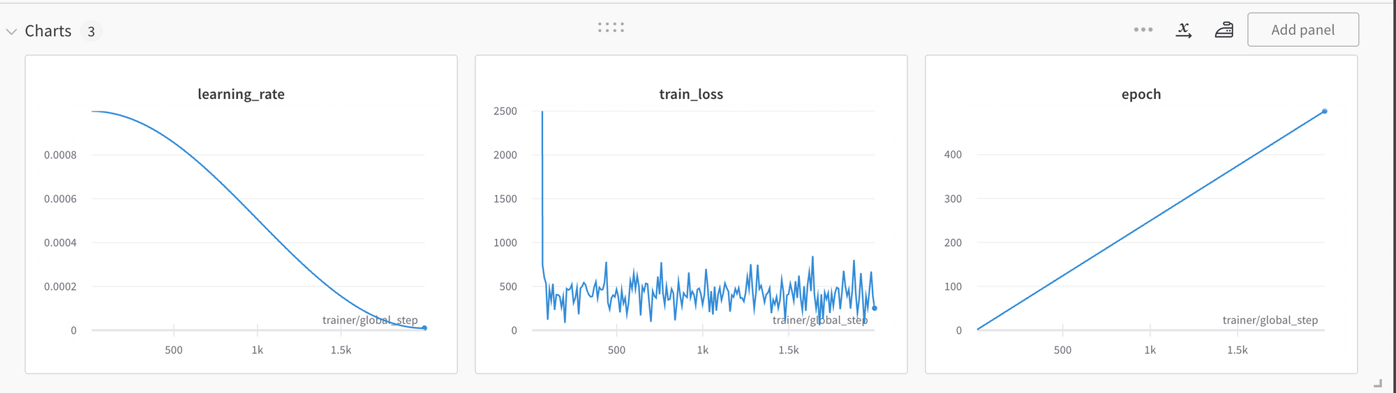
After 54 epochs the training loss (Mean Squared Error) has converged to a very low number (close to 1.0).  This

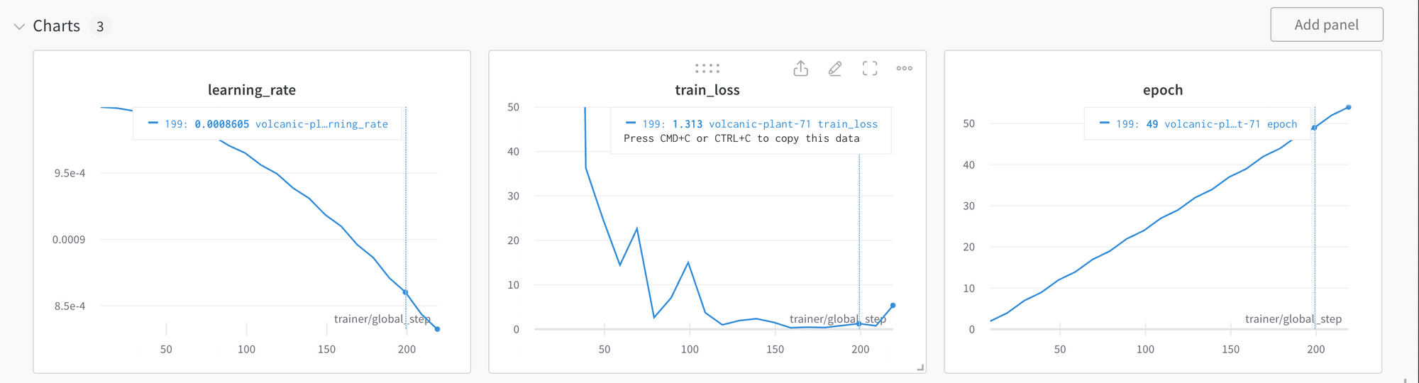
Revisiting some design decisions

Should we train from scratch vs using a pre-trained network?  According to this reddit thread the consensus is that training from scratch on with synthetic datasets followed by fine-tuning works better than transfer learning on pre-trained  networks.

However, I initially I tried training from scratch, but the network could not handle rotations.

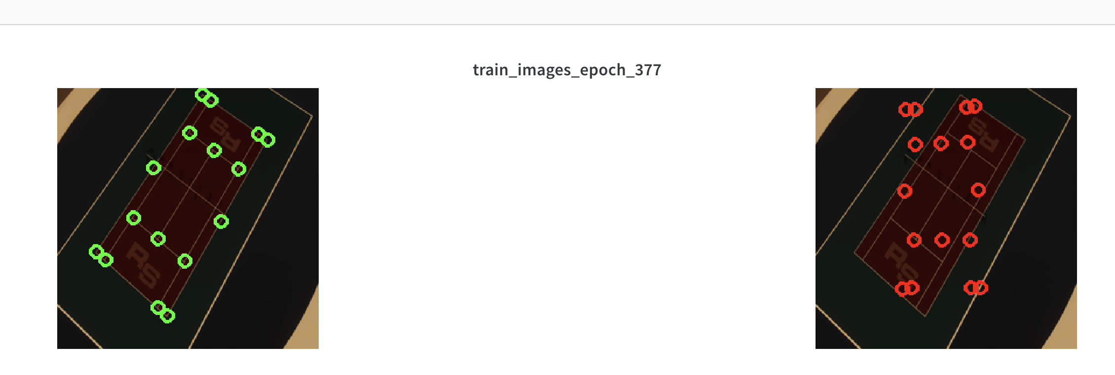
and the loss did not appear to converge even after 400+ epochs:

Some ideas on why this didn't work:

1. Serious bug - this seems to be the case, because in later parts of this blog series training from scratch yielded reasonable results
2. Not enough data samples
3. Not enough variety within data samples

You might also be wondering, when using a pre-trained network, shouldn't the images be normalized?

With VGG16, since it doesn't have any batchnorm layers, the answer appears to be yes.  Going forward I will add this to the dataset class:

        # Normalize the image on the pretrained model's mean and std
        normalized_image = torchvision.transforms.Normalize(
            mean=[0.485, 0.456, 0.406],
            std=[0.229, 0.224, 0.225])(resized_image)

Recap

In this part we've used transfer learning to achieve an MSE loss of ~ 1.0 pixels on a small synthetic dataset.

We've also built visualizations to help assess the network progress during training.

In the part 3 we'll make the dataset a bit harder and introduce occluded keypoints, and improve the network to handle these.