Tennis court line detector: Part 5, test on unseen tennis court

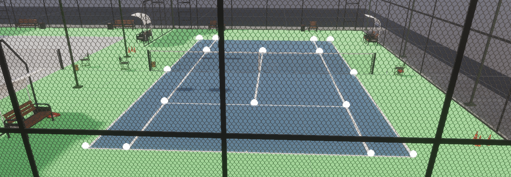
In part 4 we got fairly good results on the validation set. In this part, we'll try to run the validation on this new synthetically generated tennis court, which is not present in the training data.
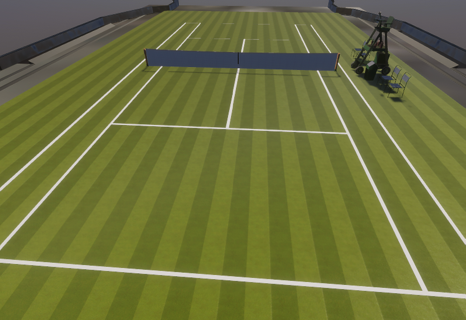
Here's a 3rd tennis court model, this time with a grass surface.

For the test set, I generated 150 images of this court with random lighting and rotations.
Hacking the test set into the validation set
Since the code already displays visual annotations of the predictions on the validation set, let's be a bit lazy and do a trick to:
- Train on the previous train + validation sets
- Validate on the test set
    # Change the split so that 99.9% of the train/validation data is used for the training dataset
    train_dataset, val_dataset = train_test_split(dataset, test_size=0.01, random_state=42)

    # Use the test dataset as validation dataset, override split dataset
    val_dataset = TennisCourtDataset(
        data_paths=test_solo_dirs,
    )

	# Create the wrapped datasets as before
    train_dataset_wrapped = TennisCourtDatasetWrapper(train_dataset, transform=transform)
    val_dataset_wrapped = TennisCourtDatasetWrapper(val_dataset, transform=A.Compose([]))
Run the model on new court
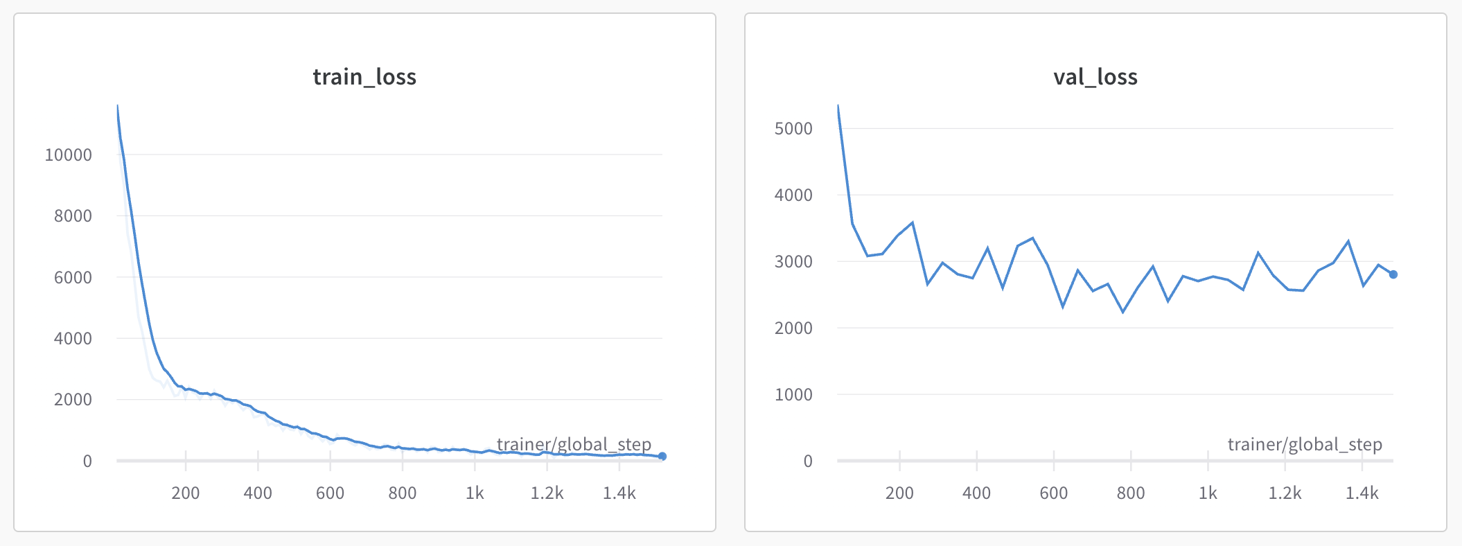
The results are .. terrible.
The validation loss hits a wall at 3000

and inspecting the resulting predictions show how far off the predictions are:

The model is completely overfitting the training data and not finding features that generalize well to unseen data.
Ideas on why the model is not generalizing
Here are what I believe to be the core issues that are preventing the model from generalizing to unseen tennis courts:
- Not enough training data (~1200 images) for training from scratch
- Not enough variety of training data (2 tennis courts, only certain angles and lighting)
- Test on a model with a grass surface, with no instances of a grass surface in the training data
If you have other ideas on what's going wrong, send me a DM on twitter (or @ me).
Resources (code and data)
- Code: https://github.com/tleyden/tennis_court_cnn
- Data: training zip (3.4GB), test zip (95 MB)
Conclusion and take aways
Use Unity Perception more efficiently
Unity Perception is a powerful toolkit for generating synthetic data, however at least for certain problems there are still challenges for creating large and high variety datasets. As a Unity novice, I wasn't able to figure out a way to efficiently do this.
Rather than juggling separate unity scenes for each tennis court, and having to go through all the steps to do the keypoint annotations, it would be better to have a single tennis court and programmatically alter aspects of the court like the texture and other aspect of the appearance.
Debug the network by visualizing features
CNNs are a bit of a black-box, which makes it challenging to try to figure out what's going on when they don't give the desired results.
It would be interesting to visualize the CNN features. My guess is that in this case, the features would be unrelated to the features you (as a human) would expect or want the network to be learning.
Trade offs of materializing the train/test split
There are two ways to write the train/test split code:
- Using scikit-learn's
train_test_split - Using pytorch's
random_split
The scikit-learn approach requires a much higher memory footprint, because it will preload the entire image set in memory. However, it will then train much faster.
Switching from pytorch augmentations to Albumentation augmentations is tricky
Pytorch augmentations work with pytorch tensors, and require no additional pre-processing. However Albumentations require numpy arrays, so the dataset code needs to be reworked accordingly.
In retrospect, since Albumentations offers more powerful augmentations, and runs much faster, it's probably better to just start with Albumentations and avoid having to rework the code.
Applying augmentations to the training set was harder than expected
I was expecting to be able to apply augmentations to only the training set with a one-liner, like maybe passing the transformations into the training data loader but not the validation data loader. Unfortunately, this is done via the pytorch dataset subclass, which is shared by both the training and validation loader.
The best approach I could find was to create two dataset objects:
- The generic dataset object that would read the full dataset that could be passed to sklearn's
train_test_splitfunction. It would read images into memory, but not apply any transformations other than resizing. - Create a separate "wrapper" dataset that could call the underlying generic dataset object, and conditionally invoke transformations for training data (only)
Augmentations would have been better done via Unity Perception
At one point I applied a warping augmentation, but then quickly realized that the keypoint coordinates would not longer correspond to the correct image coordinates. Had these augmentations been at the Unity layer, then the keypoint 2D pixel coordinates would have been automatically adjusted.
This seems like a much more robust approach to generating a high variety dataset than image level augmentations.
View-dependent keypoints was limiting
Because the keypoints had notions of "front" and "back" baked in, this limited the number of views that could be generated. For example, if the court was rotated too much by the Unity Perception rotation randomizer, you would end up with conflicting annotations where some images had front labeled keypoints in the back and vice-versa.
Since my understanding is that keypoints must be unique, I didn't see a better way.
Weights and Biases was excellent for visualizing the results
This required two steps:
- Write some opencv code that could superimpose keypoint annotations on images
- Save the generated images to Weights and Biases so they could be visualized in their dashboard
I felt this was well worth the effort - it helped show where the network was doing well and where it was struggling.
Constraining the output range might be helpful
For example, the raw logits could be scaled with the sigmoid function to get squashed between 0 and 1, then rescaled back to the 224x224 image for visualization purposes.
Why would this be useful? This would effectively constrain the output range to 0-224, versus the current code that could produce any arbitrary floating point number as an output.
Leveraging prior knowledge about tennis courts might be helpful
The current approach builds a model that predicts raw keypoint locations, but it does not take into account the prior knowledge about tennis courts, which have very precise dimensions and fixed relative positions of keypoints.
Instead of predicting keypoints, it might be better to take the following approach:
- Have the notion of a "canonical court" with the standard tennis court ratios, scaled to a certain factor.
- Predict the quaternion that is required to scale, rotate, and translate the canonical court so that it aligns with the actual tennis court image.
It would be another form of constraining the problem to make it easier for the network to learn, since there are less degrees of freedom to consider here.
Mixing continuous and categorical variables requires careful treatment
Categorical variables need their own "head" and should not be mixed with continuous variables, since they each have their own loss functions.
If possible, group the related categorical variables into a single head rather than unnecessarily having separate heads. This may require "unrolling the batches" as was demonstrated in part 3.
If you enjoyed this blog post or have any other feedback, send me a DM on twitter.
Happy (deep) learning and hacking!
